Welcome to the third day of the FAS Informatics Bioinformatics Tips and Tricks Workshop!

If you're viewing this file on the website, you are viewing the final, formatted version of the workshop. The workshop itself will take place in the RStudio program and you will edit and execute the code in this file. Please download the raw file here

Today we're going to continue our tour and explanation of common genomics file formats and their associated tools, starting with GFF files, which are typically used to store gene annotations. We'll then talk about VCF files, which are used to store variants.

In the second half of the workshop, we'll introduce some basic concepts about bash scripting, in preparation for day 4 which will be all about scripting.

Setting up our link to the data files

Like previous days, we'll make a link to the source data files for the day. Though for the beginning of the workshop we'll still be working with day 2 data in your data2 folder.

Run the code block below to create your link for the day 3 data:

mkdir -p data3
ln -s -f /n/holylfs05/LABS/informatics/Everyone/workshop-data/biotips-2023/day3/* data3
# ln: The Unix link command, which can create shortcuts to folders and files at the provided path to the second provided path
# -s: This option tells ln to create a symbolic link rather than a hard link (original files are not changed)
# -f: This option forces ln to create the link

ls -l data3
# Show the details of the files in the new linked directory

GFF

The format for encoding information about genic regions (commonly called a genome annotation) is the GFF format. GFF stands for General Feature Format. The specification has undergone two major revisions, with the most recent (and commonly-used) being GFF3. There is a related format, the GTF format, which stands for General Transfer Format but it is very similar to GFF (being an extension to GFF2) and not as commonly used, so we will only talk about GFF files today. While GFF/GTF files are commonly used to store information about genes, they can store any location information, and share some similarities with bed files (which we discussed last week).

GFF files are also tab delimited files, with each row in the file referencing a particular region in the genome and each column a piece of information about that feature This probably sounds similar to the bed format, but contains more required columns. GFF files by definition have the following columns:

Chromosome or assembly scaffold ID: The sequence name in the genome assembly file
Annotation source: The name of the data source or program that annotated this feature
Feature type: A categorical name for the type of feature defined in this row (e.g. "gene", "transcript", "exon")
Feature start coordinate: The (1-based) start position of the feature defined in this row
Feature end coordinate: The end position of the feature defined in this row
Score: The score of the feature if quality is assessed during annotation, otherwise .
Strand: Either + (forward strand) or - (reverse strand)
Frame: For coding exons, this indicates the frame as either 0, 1, or 2
Attribute: A semi-colon separated list of any other information related to the feature defined in this row

For more detailed information on GFF files, see the following links:

Let's take a look at a GFF file and talk about it a bit.

Run the code block below to view the first few lines of a GFF file. Note that this is in Day 2's data folder.

grep -v "biological_region" -m50 data2/Macaca_mulatta.Mmul_8.0.1.86.chr.gff3
# grep: The Unix string search command
# -v: This option tells grep to print lines that DO NOT contain the following string
# "biological_region": The string to search for in the provided file - we just don't want to display these for this demonstration
# -m50: This option tells grep to only display the first 50 matches

We'll just point out a couple of things. First, this file also has a header, like a BAM file, though this is not required for GFF files (note that the ##gff-version directive is required by the GFF3 specification, though in practice many parsers accept GFF3 files without it). In general, the GFF format is less standardized than others we've gone over in the workshop. Next you'll note that columns 1, 3, and 4 are the same three columns (ALTHOUGH WITH DIFFERENT INTERVAL ENCODING) that define a bed file, so GFF files are (sort of) easy to convert to bed files, though with loss of information. This also means some bedtools programs can process GFF files as well.

Features in a GFF file are generally nested: genes are comprised of transcripts and transcripts are comprised of exons. All of these features are encoded in this file and are usually linked to each other by IDs in the last column, though this is not always standardized. This can make the strand column slightly confusing to work with for features nested under the same parental feature. For features on the positive strand (+), it is straightforward: they are ordered by start coordinate. For features nested under the same parental feature on the negative strand (-) though, the correct order is the reverse sorting by the end coordinate. Many of the tools we work with will consider and correct for strand, but it is always a good thing to consider if you ever parse GFF files on your own.

Because of all the quirks with GFF files, there are many tools out there to help process and analyze them, such as gffread and AGAT. We won't be demonstrating these today though.

In the previous workshop, we demonstrated how to use awk, a scripting language that is very useful for processing text. Similarly to how we used awk for BED files, we can also use it for GFF files.

Run the following piece of code in the terminal:

awk 'BEGIN{FS="\t"} $3=="gene"{print}' data2/Macaca_mulatta.Mmul_8.0.1.86.chr.gff3

Let's go through each piece of the above command to refresh our memories: - We use the BEGIN pattern to tell awk to execute that command before any lines are read in the file
- We set the field separator (i.e. FS) as a tab character, as GFF files are tab-delineated
- We provide the pattern $3=="gene", meaning that the following code will only execute when the third column (indicated by $3) exactly matched the string gene - print simply prints the line (only when the preceding pattern is true)

In other words, this code simply prints all lines in the GFF file that are a gene annotation! Now let's get a little more advanced:

In the previous workshop, we demonstrated how to use awk, a scripting language that is very useful for processing text. Similarly to how we used awk for BED files, we can also use it for GFF files.

Run the following piece of code in the terminal:

awk 'BEGIN{FS="\t"} $3=="gene"{print}' data2/Macaca_mulatta.Mmul_8.0.1.86.chr.gff3

Let's go through each piece of the above command to refresh our memories: - We use the BEGIN pattern to tell awk to execute that command before any lines are read in the file
- We set the field separator (i.e. FS) as a tab character, as GFF files are tab-delineated
- We provide the pattern $3=="gene", meaning that the following code will only execute when the third column (indicated by $3) exactly matched the string gene - print simply prints the line (only when the preceding pattern is true)

In other words, this code simply prints all lines in the GFF file that are a gene annotation! Now let's get a little more advanced:

Exercise: In the code block below, write an awk command that counts the number of genes in the macaque annotation. Be sure to only check the feature name column (third column) because any feature that has a gene as a parent will also have a "gene id" in the last column that would return that line if it was searched for the string "gene". Also be sure to only get exact matches for the word "gene", else pseudogenes might be included in the count:

ExerciseSolution

## Write awk command to count the number of genes in the macaque annotation
# data2/Macaca_mulatta.Mmul_8.0.1.86.chr.gff3

## Write awk command to count the number of genes in the macaque annotation

## Write awk command to count the number of genes in the macaque annotation
# data2/Macaca_mulatta.Mmul_8.0.1.86.chr.gff3
awk 'BEGIN{g=0} $3=="gene"{g++}; END{print g}' data2/Macaca_mulatta.Mmul_8.0.1.86.chr.gff3
## Write awk command to count the number of genes in the macaque annotation

BONUS Exercise: In the code block below, write an awk command that calculates the average number of transcripts per gene in the macaque annotation. This requires initializing 2 counter variables at the beginning and searching for 2 patterns separately within your awk script, and then doing some math at the end:

ExerciseSolution

## Write awk command to calculate average number of transcripts per gene
# data2/Macaca_mulatta.Mmul_8.0.1.86.chr.gff3



## Write awk command to calculate average number of transcripts per gene

## Write awk command to calculate average number of transcripts per gene
# data2/Macaca_mulatta.Mmul_8.0.1.86.chr.gff3
awk 'BEGIN{g=0;t=0} {if($3=="gene"){g++};if($3=="mRNA"){t++}} END{print t, g, t/g}' data2/Macaca_mulatta.Mmul_8.0.1.86.chr.gff3

awk 'BEGIN{g=0;t=0} $3=="gene"{g++}; $3=="mRNA"{t++} END{print t, g, t/g}' data2/Macaca_mulatta.Mmul_8.0.1.86.chr.gff3
## Write awk command to calculate average number of transcripts per gene

Comparing intervals - mixing GFF and bed files

Last week, we talked about bed files, and some tools to work with them, especially the program bedtools. The bedtools program can also work with GFF files natively. We'll return to the macaque SV dataset from last week for an example.

In the context of our macaque SVs, a natural question would be how many of the mutations affect genic regions, and may therefore affect some cellular function. To know this, we'll compare the SVs in our .bed file to the gene annotations in our .gff file.

`bedtools intersect`

So, how many of our SVs in our macaque population overlap with genes? For this we can use bedtools intersect, which takes two interval files (either bed or GFF) and calculates how many of the features overlap. Even though it takes GFF as input, we need to parse out the gene coordinates only.

Run the code block below to retrieve only the genes from the macaque annotation GFF file:

awk 'BEGIN{OFS="\t"} $3=="gene"{print "chr"$0}' data2/Macaca_mulatta.Mmul_8.0.1.86.chr.gff3 > macaque-genes.gff
# awk: A command line scripting language command
# '' : Within the single quotes is the user defined script for awk to run on the provided file
# > : The Unix redirect operator to write the output of the command to the following file

head macaque-genes.gff
# Display the first few lines of the new file with head

Note that we had to add the "chr" prefix to the beginning of the line. This is because the chromosome names are different between the two files. ID mismatches like this are a common cause of problems when working with different files from the same assembly.

Now we can get the overlaps between genes and SVs in our sample of macaques.

Run the code block below to use bedtools intersect to get the overlapping regions between two interval files:

bedtools intersect -a data2/macaque-svs-filtered.bed -b macaque-genes.gff > macaque-svs-genes-intersect.bed
# bedtools: A suite of programs to process bed files
# intersect: The sub-program of bedtools to execute
# -a : The first interval file to check for overlaps
# -b : The second interval file to check overlaps

wc -l data2/macaque-svs-filtered.bed
wc -l macaque-svs-genes-intersect.bed
# Use wc -l to count the number of lines in the original bed file and those in the bed file that overlaps with genes

Ok great, we've got only the SVs that overlap with genes in the macaque genome. Let's take a look at this file.

Run the code block below to view the first few lines of the bed file with SVs that overlap with genes:

head macaque-svs-genes-intersect.bed
# Display the first few lines of the bed file containing SVs that overlap with genes

Exactly the same format as the input bed file, just with fewer lines. bedtools intersect can add additional columns with more information about the overlap and overlaps can be defined more clearly. Let's try it out.

Exercise: *Read the documenation of bedtools intersect and do the following. Don't save the output to a file, just pipe it to wc -l:

Count only the SVs that DO NOT overlap with any genes.

Count only SVs that have at least 90% of their sequence overlapping a gene.

Count only SVs that have at least 90% of their sequence overlapping a gene AND for which that overlap also encompasses at least 90% of the gene.

ExerciseSolution

# data2/macaque-svs-filtered.bed

## Count SVs that DO NOT overlap with genes

## Count SVs that DO NOT overlap with genes


## Count SVs that have at least 90% of their sequence overlap with a gene

## Count SVs that have at least 90% of their sequence overlap with a gene


## Count SVs that have at least 90% of their sequence overlap with 90% of a gene's sequence (reciprocal overlap)

## Count SVs that have at least 90% of their sequence overlap with 90% of a gene's sequence (reciprocal overlap)

# data2/macaque-svs-filtered.bed

## Count SVs that DO NOT overlap with genes
bedtools intersect -v -a data2/macaque-svs-filtered.bed -b macaque-genes.gff | wc -l
## Count SVs that DO NOT overlap with genes

## Count SVs that have at least 90% of their sequence overlap with a gene
bedtools intersect -f 0.9 -a data2/macaque-svs-filtered.bed -b macaque-genes.gff | wc -l
## Count SVs that have at least 90% of their sequence overlap with a gene

## Count SVs that have at least 90% of their sequence overlap with 90% of a gene's sequence (reciprocal overlap)
bedtools intersect -f 0.9 -r -a data2/macaque-svs-filtered.bed -b macaque-genes.gff | wc -l
## Count SVs that have at least 90% of their sequence overlap with 90% of a gene's sequence (reciprocal overlap)

bedtools intersect can also output the actual features that are overlapped with the amount of overlap with the -wo option.

Run the code block below to perform an intersect between macaque SVs and genes with the -wo option:

bedtools intersect -wo -a data2/macaque-svs-filtered.bed -b macaque-genes.gff | head
# bedtools: A suite of programs to process bed files
# intersect: The sub-program of bedtools to execute
# -wo : A bedtools intersect option that specifies to write both features and the number of overlapping bases to the output file
# -a : The first interval file to check for overlaps
# -b : The second interval file to check overlaps
# | : The Unix pipe operator to pass output from one command as input to another command

VCF files

Another important type of genomic coordinate file is the VCF file, or variant call format file. This is another tab-delimited file that contains variants between a single genome or a sample of genomes and a reference genome. These variants can include single nucleotide changes, small insertions and deletions, or even larger structural variants. The most common type of variation you'll see in a VCF file are the single nucleotide ones, so the content of a VCF file is commonly referred to as SNP calls.

We'll now be working with a VCF file that contains SNP data from some Amazon molly (Poecilia formosa), a freshwater fish. The original data consists of hundreds of thousands of SNPs across the molly genome among 16 individuals, but we'll be looking only at SNPs on a single scaffold today (about 100,000).

Let's take a look at our file and explain a bit about the format.

Run the code below to view the beginning of our VCF file:

head -n 43 data3/poeFor_NW_006799939.vcf 
# head: A Unix command to display the first few lines of a file
# -n 43: This tells head to display exactly the first 43 lines of the provided file

So what we see here at the top of the file is the header of the VCF. Much like headers in BAM and SAM files, headers in VCF files contain information about how this file was created and the contents of the file. For example, the lines that begin with ##FORMAT describe the contents of a particular column of the file, while the lines begin with ##FILTER describe what the filter labels in the Filter column mean. Unlike the headers in BAM and SAM files, which begin with the @ character, the headers in a VCF file begin with the ## string (like GFF files).

Now that we know a bit about the header, let's look at the actual content of the file, the tab-delimited rows containing SNP calls.

Run the code below to view the beginning of our VCF file while skipping header lines:

grep -v "##" data3/poeFor_NW_006799939.vcf | head -n 2
# grep: The Unix string search command
# "##": The string to search for in the provided file - we just don't want to display these for this demonstration
# head: A Unix command to display the first few lines of a file
# | : The Unix pipe operator to pass output from one command as input to another command
# -n 2: This tells head to display exactly the first 2 lines of the provided file

The first line here, beginning with a single # shows us the names of the columns, which may be referred to in the file header like we saw above. Each subsequent line represents one variant relative to the reference genome, with the following column definitions:

CHROM: The chromosome or assembly scaffold in the reference genome.
POS: The (0-based) position of the variant in the reference genome.
ID: A name for the variant. If the variant has no name, just the . character.
REF: The allele in the reference genome.
ALT: The alternate allele in the the sample.
QUAL: The quality score of the variant call. How this is calculated depends on the variant calling program.
FILTER: The filter label for the current variant. If the variant isn't filter, this will be PASS (or sometimes .).
INFO: Additional info for the current variant. Usually a semi-colon (;) delimited list of information.
FORMAT: A colon (:) delimited list of the keys for the information in the subsequent columns. These keys are defined in the file header. 10+. SAMPLE GENOTYPES: Each subsequent column contains a colon (:) delimited list that follows the keys in the FORMAT column for the genotypes of the samples. Each column corresponds to one sample with the name being the column header.

The genotypes are encoded in the sample columns with the GT key. In this file, it is the first entry. For example, with the keys defined in column 9, the genotype of the first sample:

./.:0,0:0:.:.:.:0,0,0:.

means that the GT (GENOTYPE from the header) is ./., the AD (ALLELIC DEPTH) is 0,0, the DP (DEPTH) is 0, and so on.

Genotypes use the following syntax, with 0 being the reference allele and 1 being the alternate allele:

0/0 means this sample is homozygous for the reference allele.
0/1 or 1/0 means this sample is heterozygous for the reference allele (0) and the alternate allele (1).
1/1 means this sample is homozygous for the alternate allele.
. is used for missing; this site was not genotyped for this individual, which happens to be the case for the sample outlined above.

For VCF files with multiple samples (like this one), sites can have more than two alleles, in which case the genotypes 0/2 or 0/3 or 2/2 may be seen.

There are many quirks to VCF files, but they are also highly standardized, so if you find yourself working with them be sure to read the very detailed specifications here:

VCF file specs

Note

Note that the binary version of VCF files are BCF files, usually with the .bcf file extension. BCF files are more efficient to read than VCF files, and are typically compressed.

There are a myriad of ways to use and analyze a VCF, but for general processing of them, we will use bcftools. bcftools falls under the same development umbrella as samtools and thus shares much of the same usage and underlying philosophy to act like a native Unix command. It was preceded by vcftools, which still retains some useful functionality, but is no longer developed.

bcftools

Much like bedtools, bcftools has a wide range of functions so we won't be able to get to everything today. Be sure to read the documentation to find out if it can accomplish the task you need with your VCF or BCF file.

One of the most basic things you can do to a file is to view it. Indeed, looking at your data is an important part of each step of a bioinformatics workflow.

Like samtools, bcftools has a dedicated view command.

Exercise:

Run the code below to view the top of the Amazon molly VCF file.

Edit the bcftools view command to exclude the header from the output.

ExerciseSolution

## Use the view command to display the VCF file, then edit it to exclude the header
## data3/poeFor_NW_006799939.vcf

## NOTE: ignore the "cannot write" error! This is just an artifact of our setup for the workshop today.

## Use the view command to display the VCF file, then edit it to exclude the header
## data3/poeFor_NW_006799939.vcf
bcftools view -H data3/poeFor_NW_006799939.vcf | head -n 10
## NOTE: ignore the "cannot write" error! This is just an artifact of our setup for the workshop today.

So view acts much the same way as the Unix command cat, but has specific functionality for the VCF format, and also handles compressed BCF files natively.

One useful function when viewing files is to be able to subset or filter them. We've provided a file that lists the sample IDs for a made-up population and can use bcftools view to extract genotypes from specific samples.

Run the code below to extract SNPs only from a subset of samples:

cat data3/pop1.txt
# cat: A Unix command that displays the contents of a file in the Terminal
# This is just to see the pop1.txt file

bcftools view -S data3/pop1.txt -H data3/poeFor_NW_006799939.vcf | head
# bcftools: A suite of programs to process VCF files
# view: The sub-program of bcftools to execute
# -S : A bcftools view option that specifies to only extract genotype columns from the samples listed in the provided file
# -H : A bcftools view option that specifies to exclude the VCF header from the output
## NOTE: ignore the "cannot write" error! This is just an artifact of our setup for the workshop today.

A note about subsetting

This can be very handy, but be warned - the INFO fields are not automatically recalculated, and will no longer be correct once you remove some individuals. In general, the INFO column and its information displays information about the site while the FORMAT fields display information about each sample.

SNP density with `bcftools` and `bedtools`

Many of the tools we've demonstrated, samtools, bedtools, bcftools, are general purpose tools for basic processing and manipulation of specific file formats used in genomics. Many of the tasks they do could be done with native bash commands, but that would require a lot of piping and probably some custom scripting on uncompressed files. However, if you really start to get to know these tools and their versatility, you can do some more advanced analyses purely with them. Let's demonstrate by calculating SNP density across 100k windows the specific 7 Mb scaffold we are working with from the Amazon molly genome.

To do this, we'll need:

The .fai index file of the Amazon molly genome, which we have already generated.
A bed file with the coordinates of the 100 kilobase windows in the scaffold
A VCF file with Amazon molly SNPs, which we have provided.

Since we've already downloaded the genome and generated the index file, let's start with the second one, getting the window coordinates. We can do this easily with the bedtools getwindows command:

Run the code below to generate a bed file with 100kb windows in the Amazon molly genome:

bedtools makewindows -g data3/poeFor_NW_006799939.fasta.fai -w 100000 > poeFor-windows-100k.bed
# bedtools: A suite of programs to process bed files
# makewindows: The sub-program of bedtools to execute
# -g : A genome size file, which needs two columns, the scaffold/chromosome name and the size of that feature
# -w : The size of the windows to partition each scaffold in -g into
# -b : The second interval file to check overlaps
# > : The Unix redirect operator to write the output of the command to the following file

head poeFor-windows-100k.bed
# Display the first few lines of the bed file containing windows

Now, we can use bedtools intersect, which also works with VCF files, to count how many SNPs appear in each window.

Exercise: Use bedtools intersect to count the number of SNPs in each 100kb window in the Amazon molly genome. You will need to look in the help menu of bedtools intersect to find the right option to output a column with the number of overlaps per region! Save this file as poeFor-windows-100k-snps.bed.

ExerciseSolution

## Write a bedtools intersect command to count how many SNPs overlap each 100kb window in the molly genome
## data3/poeFor_NW_006799939.vcf
## poeFor-windows-100k.bed

## Write a bedtools intersect command to count how many SNPs overlap each 100kb window in the molly genome

head poeFor-windows-100k-snps.bed
# Display the first few lines of the bed file containing windows and overlapping SNPs

## Write a bedtools intersect command to count how many SNPs overlap each 100kb window in the molly genome
## data3/poeFor_NW_006799939.vcf
## poeFor-windows-100k.bed
bedtools intersect -c -a poeFor-windows-100k.bed -b data3/poeFor_NW_006799939.vcf > poeFor-windows-100k-snps.bed
## Write a bedtools intersect command to count how many SNPs overlap each 100kb window in the molly genome

head poeFor-windows-100k-snps.bed
# Display the first few lines of the bed file containing windows and overlapping SNPs

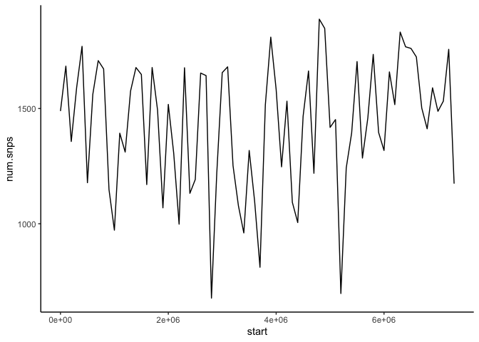
BONUS Exercise: If you attended the R workshop last week or know R already, use the code block below to read in the file we just generated with SNPs per 100k window and plot the density along this scaffold.

ExerciseSolution

library(tidyverse)
# Load the tidyverse

## Write code in R to plot SNP density across the scaffold in our bed file
# poeFor-windows-100k-snps.bed

library(tidyverse)

# Load the tidyverse

## Write code in R to plot SNP density across the scaffold in our bed file
# poeFor-windows-100k-snps.bed
am_snps = read_tsv("poeFor-windows-100k-snps.bed", col_names=c("scaffold", "start", "end", "num.snps"))
# Read the bed file containing 1Mb windows and number of SNPs per window, and name the columns

snp_plot = ggplot(am_snps, aes(x=start, y=num.snps)) +
# Initialize a ggplot grob and load the data and aesthetics into it and store it as the snp_plot object

  geom_line() +
  # Plot the provided data as a line graph

  #facet_wrap(~scaffold, scales="free") +
  # Split the plot by scaffold

  theme_classic()
  # Set a different theme
## Write code in R to plot SNP density across the scaffold in our bed file

print(snp_plot)

Scripts

So far, we've been focused on interactive analysis of small files. However, in real bioinformatics work, you will likely find yourself with many samples that you want to run the same commands on. And often these commands can require significant compute time, such that you want to be able to run these commands non-interactively. As nice as these markdown notebooks are for teaching and data exploration, they are not the ideal format for this task. Instead, what we want are scripts.

A bash script (like an R script, if you attended the R workshop earlier), is just a text file that executes a series of commands in order. Bash scripts can get exceedingly complicated, but today we are just going to introduce a few basic concepts.

We are ultimately going to make a script that takes as input a VCF file and one or more bed files, and reports as output the average SNP density in regions of the genome inside bed intervals. Let's start simple.

Note

To follow every step for this instructor version, we provide a separate script for each step titled snp-density-N.sh. In the student version you updated a single script, snp-density.sh. These can be downloaded individually at https://harvardinformatics.github.io/workshops/2023-fall/biotips/snp-density-0.sh and by incrementing the number in the filename, (e.g. -0.sh, -1.sh, etc)

Using the file menu, go to New file --> Shell script and create a new file. Call it snp-density-0.sh.This is going to be our script in a new tab of our text editor, that we will modify as we go.

The first thing we need to do is a little bit of shell magic to get the shell to treat the script we are writing as a command. This is called a shebang (#!) and basically says "run the script with the following interpreter". Type the following line at the top of your script:

#!/bin/bash

This means that when we run snp-density-0.sh on the command line, the commands in the script will be interpreted as shell commands.

We need to do one more thing, which is make our script executable. We'll use the chmod command for this.

In the Terminal below, make sure you are in the same directory as your script file, and then type the following command.

chmod +x snp-density-0.sh

We now have a script we can run.

Try running your (empty) script. Note that the ./ specifies the relative path to the script, and means "execute the script snp-density.sh in the current working directory". If omitted, you'll get a "command not found" error.

chmod +x snp-density-0.sh
# Make the script executable

./snp-density-0.sh
# ./ : Execute the following file as a shell script

However, nothing will happen if we do, since there are currently no commands in the file to run.

Exercise: In order to have our shell script do anything, we need to put some commands in it. 1. Copy the bedtools intersect command from above into the script, but don't write the output of the command to a file

Now, try running your script again, piping the output to head.

Try running your script.

chmod +x snp-density-1.sh
# Make the script executable

./snp-density-1.sh | head
# ./ : Execute the following file as a shell script

Now, all the commands to create our snp density windows are in the script. Let's say we wanted to calculate the average snp density across all windows, with awk. Here is an awk command that can do that:

./snp-density-1.sh | awk 'BEGIN{snps=0; lens=0} {snps+=$4; lens+=$3-$2} END{print snps/lens}'

If we run this, we should get a number now.

Let's add the awk command to our script now, so that when we run snp-density.sh the output will be a number with the average snp density across windows.

./snp-density-2.sh

However, we have a problem. Ideally, we'd like to be able to do this calculation on any VCF file and any bed file. Right now those files are hard-coded, which means to change what file the script operates on requires changing the script.

To make our script flexible, we need to introduce the concept of variables. We've seen this in awk commands; we can also create variables in the shell. We do this just by assigning something (text or the output of a command, usually) to a string.

Run the commands in the block below in the Terminal to create a variable called TEXT, and print it out with the echo command.

TEXT="Hello World!"
# = : Assign the variable name on the left to the value on the right

echo $TEXT
# echo: A Unix command that simply prints the provided input to the screen
# $ : A symbol that the shell understands to mean that the following is the name of a variable

Note that when we access what is stored in the variable we use the $ notation, but we don't use this when we assign to a variable. Note also we cannot have spaces before or after the equal sign or the shell will thing we are trying to run the TEXT command, not create a variable called TEXT.

Exercise: 1. Modify our shell script, snp-density.sh, so that it includes two variables, one called VCF and one called BED. For now, define these in the second and third lines of the script with the paths to the BED file and the VCF file we currently have. 2. Replace the hard-coded file names in the bedtools intersect command options -a and -b with the BED and VCF variables. 3. In the code block below run your script again and make sure it still works.

chmod +x snp-density-3.sh
# Make the script executable

./snp-density-3.sh
# ./ : Execute the following file as a shell script

You should get the same answer as before.

Note that right now, we aren't actually changing anything, we've just moved the files we are going to operate on to the top of the script, but we still would need to change the script each time we run it on different files. To make our script more general (able to take various inputs more easily), we should have a way to change the input file without having to edit the script. The way to do this is with command line options. You've seen this a lot in the tools we've run up to this point. For instance, when we run almost any shell command, it requires a filename, e.g.:

head poeFor-windows-100k.bed

In this case, the file name poeFor-windows-100k.bed, is a command line option, also known as a command line argument or just option, argument, or parameter. Commands and scripts can take multiple arguments. Some are positional, meaning that the way they are read into the program depends on their placement in the command. Others have specific flags, meaning the way they are read into the program depends on the flag they come after in the command. For instance:

head -n 20 poeFor-windows-100k.bed

This is a command that hopefully looks pretty understandable to you by now. This command, head has two command line options as we've written it:

A flag, -n 20, which changes the number of lines the command displays. Internally, this sets the value of some variable to a different number.
A positional argument, the file name poeFor-windows-100k.bed, which is the last listed argument. Again this internally sets the value of some variable to the path to that file (actually, for most bash commands, the first un-flagged option is usually reserved for the file name).

Well, we can modify our script to take input from the command line as well. Shell scripts have access to special variables that can be used to create simple, positional, command line options. Specifically, the variables $1, $2, $3, etc will contain the first, second, third, etc. arguments specified after the script is called.

Exercise: 1. Modify your script to replace the path to the bed file with $1, and the path to the VCF file with $2 using positional command line arguments. 2. Run the following code block to call your script again, this time taking arguments, with the bed file first and the vcf second.

chmod +x snp-density-4.sh
# Make the script executable

./snp-density-4.sh poeFor-windows-100k.bed data3/poeFor_NW_006799939.vcf 
# ./ : Execute the following file as a shell script

If everything is working, you should get the same answer as before. But now we can give our script any bed file and any VCF file, right from the command line. Note that we don't do any error checking - if you accidentally specify a VCF file that uses a different reference genome than your bed file, nothing in the script will prevent this.

This is better, but it still requires a lot of typing if we want to run this on 10 files. If, for example, we wanted to compute SNP density separately for each chromosome, or for different interval types (e.g., genes, introns, exons), we'd have to type out each bed file separately.

We can get around this by using loops, which we'll cover next time

Setting up our link to the data files

GFF

Comparing intervals - mixing GFF and bed files

bedtools intersect

VCF files

bcftools

A note about subsetting

SNP density with bcftools and bedtools

Scripts

`bedtools intersect`

SNP density with `bcftools` and `bedtools`