Differential expression analysis of bulk RNA-seq data
 Adam Freedman
Bulk RNA-seq involves generating estimates of gene expression for samples consisting of large pools of cells, for example a section of tissue, an aliquot of blood, or a collection of cells of particular interest, such as those obtained via fluorescence-activated cell sorting (FACS). The two primary pillars of bulk RNA-seq analysis are the estimation of gene expression levels, at either the gene or isoform level (or both), and statistical analysis to identify genes or isoforms that show different levels of expression between a set of conditions or treatments of interest. This tutorial provides a brief review of expression quantification, but mostly focuses on how to perform tests for differential expression with limma. See Ritchie et al. 2015 for more details. Limma is built on a linear-modeling framework and is available as a Bioconductor package in R.
Tutorial target audience
This tutorial is designed to demonstrate best practice for implementing statistical methods on bulk RNA-seq data to test the null hypothesis that expression of individual genes does not vary between conditions. Ideally, users of this tutorial will have a working understanding of:
- how to use R , and ideally how to run it inside Rstudio
- what gene expression estimates quantify, and the methods for performing such quantification
- hypothesis testing using statistics
Getting Started
This tutorial is divided into two parts: data preparation and differential expression analysis. Data preparation converts raw sequencing data into a table of gene-level counts (also referred to as a count matrix), where rows correspond to genes and columns correspond to samples.
Data preparation typically occurs on a high-performance computing (HPC) cluster or in a cloud computing environment, because it requires more computational resources than are typically available on a personal computer. In our data preparation section, we will be using a pre-made bioinformatics pipeline from the Nextflow nf-core project. A Nextflow workflow is a set of scripts that automate the multiple steps of data preparation, leading to reproducible and portable workflows.
The differential expression analysis part of this tutorial is designed to be performed using on a personal computer using the R programming language and the limma package. This part of the tutorial involves performing statistical inference, creating figures/plots of the data, and interpreting the results.
If you are interested in following along with this tutorial but also want to go through the process of runningthe nf-core/rnaseq workflow to generate the required expression data, you will need the following:
- A set of paired-end RNA-seq fastq files from the paper by Zhao et al. (2015) PLoS Genetics , which can be downloaded from the NCBI Short Read Archive (SRA) under the accession numbers SRR1576457-SRR1576516 and collected here .
- A genome fasta file for Drosophila melanogaster and a gtf annotation file for the same species. We used the following genome fasta and gtf files.
- A current version of nextflow installed on an HPC cluster you are using (in our case, we are using the Cannon cluster at Harvard)
If you want to skip directly to the differential expression analysis part, you will need the following:
- R and RStudio installed on your computer.
- The R markdown (Rmd) file for this tutorial. Link .
- The sample sheet that relates sample IDs to experimental conditions. Link .
- The gene-level count matrix generated by the nf-core/rnaseq workflow. Link .
Quantifying expression: a brief review
In order to obtain counts of RNA abundance from fastq files, one must employ statistical methods that account for two levels of uncertainty. The first of these is identifying the most likely transcript of origin of each RNA-seq read. The second is the conversion of read assignments to a count matrix, and doing so in a way that models the uncertainty inherent in many read assignments.
While some reads may uniquely map to a transcript from a gene without alternative splicing, in many cases shared genomic segments among alternatively spliced transcripts within a gene will make it challenging (and in some cases impossible) to definitively identify the true transcript of origin. Early bioinformatics approaches to RNA-seq quantification simply discarded reads of uncertain origin, leading to substantial loss of information that undoubtedly undermined the robustness of expression estimates, and effectively precluded investigations of expression variation among alternatively spliced transcripts. Fortunately, there are now two common approaches for handling read assignment uncertainty in a way that can be leveraged by state-of-the art tools that quantify expression.
The first entails formally aligning sequencing reads to either a genome or a set of transcripts derived from a genome annotation, such that exact coordinates of sequence matches, mismatches, and small structural variations are recorded. In both of these instances, a sam (or bam) format output file is produced that describes where reads aligned to, assigns a score to each alignment, etc. Alignment directly to a genome requires using a splice-aware aligner to accommodate alignment gaps due to introns, with STAR being the most popular of these, while tools like bowtie2 can be used to map reads to a set of transcript sequences.
The second approach was motivated by potential scalability issues with performing sequence alignment, given that it is computationally intensive, and that, because sequence alignment is done separately for each sample, scaling up to thousands or tens of thousands of samples might become computationally prohibitive. This approach, called "pseudo-alignment", does not undertake formal sequence alignment but instead uses substring matching to probabilistically determine locus of origin without obtaining base-level precision of where any given read came from; it also allows for there to be uncertainty in the transcript of origin. The pseudo-alignment approach is much quicker than sequence alignment. Tools such as Salmon and kallisto employ this approach. An added bonus of pseudo-alignment tools is that they simultaneously figure out where reads come from (the first level of uncertainty) and convert assignments to counts, producing sample-level counts that can later be converted to the count matrix format takes as input by tools that perform differential expression analysis. As a result, this saves end users from having to perform quantification separately.
A different approach to converting read assignments to counts is to model assignment uncertain recorded in sequence alignment sam or bam files produced by tools like STAR and bowtie2. A popular tools for doing this is RSEM , which uses an expectation maximization algorithm to estimate counts.
Because bam files contain a lot of information that are useful for performing quality checks on your data, we believe it is worthwhile to perform sequence alignment unless it is computationally infeasible. As a result, we recommend a hybrid approach to addressing the two levels of uncertainty described above. This approach involves two steps. First, we recommend using STAR to align reads to the genome to facilitate the generation of QC metrics for individual samples. Second, we recommend using salmon to perform expression quantification, so that we can leverage its statistical model for handling uncertainty in converting read origins to counts. This is possible because salmon has an alignment-based mode that can take bam files as input. Because salmon requires that input alignments are to the transcriptome (and not the genome), we describe below an automated workflow that takes as input the fastq files for all the samples to be used in a study, performs STAR alignments, internally converts those alignments to a format useable by salmon, and produces sample-level expression outputs as well as transcript and gene count matrices.
Summary
A few key points are worth reiterating
- there are two levels of uncertainty when producing expression estimates from fastq files, the first relates to assigning reads to a transcript of origin, and the second relates to converting read assignments to counts.
- read alignment is computationally expensive, but can be important if extended quality checks on individual RNA-seq libraries are likely to be important
- pseudo-alignment is much faster tha read alignment, and can be a sensible choice when thousands of samples are being analyzed (assuming alignment-based QC metrics are not necessary)
- some tools such as
salmoncan use sequence alignments, or run pseudo-alignment directly on fastq files to produce expression estimates - neither alignment or pseudo-alignment based quantification tools generate the data matrix of counts (rows for each gene, columns for each sample) required for differential expression analysis. However the
nf-core/rnaseqworkflow (described below) will generate them, and tools likeRSEMhave utilities for creating them from a set of samples.
Quantifying expression: best practice using the nf-core/rnaseq workflow
In order to obtain a comprehensive set of quality control metrics on our fastq files, while also obtaining gene and isoform-level count matrices from Salmon's (isoform-level) quantification machinery, we use nf-core's RNA-seq pipeline, found here . nf-core is a collection of Nextflow workflows for automating analyses of high-dimensional biological data. Nextflow is a workflow language that can be used to chain together multi-step data analysis workflows, which can easily be adapted for running on high performance computing enviornments such as Harvard's CANNON cluster. The RNA-seq workflow has a variety of option to choose from, but we specifically use the "STAR-salmon" option (see the green line in the workflow diagram below). This option performs spliced alignment to the genome with STAR, projects those alignments onto the transcriptome, and performs alignment-based quantification from the projected alignments with Salmon. The workflow requires as input a specifically formatted sample sheet, a genome fasta, and either a gtf or a gff annotation file.
Click here to see the nf-core RNA-seq workflow diagram

In order to run the workflow you will need
- A sample sheet in the nf-core format
- A gtf/gff genome annotation file
- A genome fasta file
- A config file with HPC-specific settings
The nf-core sample sheet format
The sample sheet has to be in comma-separated format, with specific column headers, e.g.:
sample,fastq_1,fastq_2,strandedness
sample1,fastq/sample1_R1_fastq.gz,fastq/sample1_R2_fastq.gz,auto
sample2,fastq/sample2_R1_fastq.gz,fastq/sample2_R2_fastq.gz,auto
Here are what the column headers mean:
| Column | Description |
|---|---|
| sample | The sample ID, which will be used as the column header in the count matrix |
| fastq_1 | The path to the R1 fastq file for the sample |
| fastq_2 | The path to the R2 fastq file for the sample |
| strandedness | The strandedness of the library: "auto", "forward", "reverse", or "unstranded" |
We do not recommend using single-end data for expression analysis
While it is possible to use the nf-core RNA-seq workflow with single-end data, we do not recommend it for differential expression analysis. This is because more robust expression estimates can be obtained with short paired-end reads that are effectively the same cost per base as traditional single-end layouts, i.e. 1x75bp
See: Freedman et al. 2020, BMC Bioinformatics https://link.springer.com/article/10.1186/s12859-020-3484-z
Locations of R1 and R2 can be paths relative to the location where the workflow is being launched or absolute paths. Fastq files should be gzipped. In cases where a sample id occurs in more than one row of the table, the workflow assumes these are separate sequencing runs of the same sample and counts estimation will be aggregated across rows with the same value for sample.
While strand configuration can be manually specified, we prefer to use Salmon's auto-detect function, which will also account for cases when the set of samples include data where the strandedness is unknown (e.g. SRA accessions without detailed metadata), mistakenly specified, or where issues with reagents led to a strand-specific kit producing a library without strand specificity.
The gtf/gff genome annotation file
The nf-core ecosystem was built to work optimally with annotation files from Ensembl. In most cases, it will work with NCBI annotation files. However, for both Ensembl and NCBI, the gtf versions of the annotation files are preferred.
For NCBI annotations, the workflow will occasionally fail because there are subset of (typically manually curated) features for which there isn't a value for gene_id in the attributes (9th) column of the gtf (or gff) file. A typical error message of this type starts with something like this:
In addition, warnings, or in some cases job failure will occur if there is a value for gene_biotype, so we use an additional argument --skip_biotype_qc in our workflow that skips a biotype-based expression QC metric. This applies to both NCBI gff and gtf files.
The config file
A config file needs to be supplied that specifies the type of computational resources that gets allocated for jobs that are labelled in the workflow by their memory requirements. The config file we have successfully deployed on Harvard's Cannon HPC cluster can be found here . By default, this config will have jobs run locally on the computer/node where the job is launched. To use HPC resources, you need to specify a line at the beginning of the process block indicating the executor, and an additional line below with partition names to use. In the case of the Cannon cluster, on which jobs are scheduled by SLURM, and where we use the partitions named "sapphire" and "shared", we modify the beginning of the config file to look like this:
process {
    executor = 'slurm'
    // TODO nf-core: Check the defaults for all processes
    cpus   = { 1      * task.attempt }
    memory = { 6.GB   * task.attempt }
    time   = { 4.h    * task.attempt }
    queue  = 'sapphire,shared'
where the order of queues indicates the order of prioritization for partition selection.
Executing the nf-core RNA-seq workflow
We recommend submitting the nextflow pipeline as a SLURM job on a compute node. An example SLURM SBATCH script to launch the workflow is shown below:
#SBATCH -J nfcorerna
#SBATCH -N 1
#SBATCH -c 1
#SBATCH -t 23:00:00  # time in hours, minutes and seconds
#SBATCH -p shared      # add partition name here
#SBATCH --mem=12000
#SBATCH -e nf-core_star_salmon_%A.err
#SBATCH -o nf-core_star_salmon_%A.out
module load python
mamba activate nfcore-rnaseq

nextflow run nf-core/rnaseq \
    --input nfcore_samplesheet.csv \
    --outdir $(pwd)/star_salmon \
    --skip_biotype_qc \
    --gtf genome/mygenome.gtf \
    --fasta genome/mygenome.fna.gz \
    --aligner star_salmon \
    -profile singularity \
    --save_reference \
    -c rnaseq_cluster.config
| Option | Description |
|---|---|
--input |
The path to the sample sheet in nf-core format |
--outdir |
The path to the output directory where results will be saved |
--skip_biotype_qc |
Skip the biotype-based expression QC metric, this is necessary for NCBI gff/gtf files |
--gtf |
The path to the genome annotation file in gtf format, should be uncompressed |
--fasta |
The path to the genome fasta file, should be gzipped |
--aligner |
The aligner to use, in this case star_salmon |
-profile |
The profile to use, in this case singularity |
--save_reference |
Save the reference genome and annotation files to the output directory |
-c |
The path to the config file with HPC-specific settings, if using |
- Launching nfcore/rnaseq automatically downloads the workflow from the GitHub repository, and installs all dependencies
- The genome needs to be gzipped
- The annotation file should be uncompressed. If you opt to use a gff file then,
--gtfshould be changed to--gff - A config file should be provided that specifies compute resources for various workflow child processes
The output
The output of this workflow includes:
- the star_salmon directory, inside of which are:
- bam files resulting from sequence alignment with STAR for each sample
- gene and transcript length-scaled count tables in tsv format
- gene and transcript length tables in tsv format
- gene and transcript tables with estimates of transcripts-per-million (TPM)
- salmon.merged.gene_counts.tsv and salmon.merged.transcript_counts.tsv, which are the estimated raw counts in matrix form
- the multiqc/star_salmon directory, inside of which is multiqc_report.html, and html report compiling all of the sample-level quality metrics that are generated by the workflow.
We are now ready to perform differential expression analysis in R.
Differential expression analysis: a worked example in R
This tutorial performs differential expression analysis with R, and for the purposes of making debugging and visualization/plotting easier, we recommend using RStudio, an interactive environment that can downloaded from here .
If you want to reproduce the workflow explained below, the R markdown (Rmd) file for it can be found here . The sample sheet that relates sample IDs to experimental conditions can be found at sample_sheet , and the gene-level count matrix can be found at count_matrix .
Example data
Our sample data comprises 12 paired-end RNA-seq libraries for whole body samples of Drosophila melanogaster from two geographic regions (Panama and Maine), with two temperature treatments ("low" ane "high") for each region, featuring three biological replicates for each region x treatment combination. Previously, these data were used to look for parallel gene expression patterns between high and low latitude populations (Zhao et al, 2015, PLoS Genetics ). For this tutorial, we downloaded the fastq files for the RNA-seq libraries from NCBI's short read archive and generated the count matrices using the nf-core rnaseq workflow described above. One can either perform differential expression tests on isoform (i.e. transcript) counts or gene-level counts, i.e those aggregated across all of a gene's constituent transcripts. For this tutorial we focus on gene-level patterns of differential expression. Thus we use the count data in salmon.merged.gene_counts.tsv. In this file, The column header includes "gene_id" and "gene_name" for the first two columns, and the sample names from the sample sheet for the remaining column labels. In other words, each row in the file includes a gene id (first column), a gene name (e.g. HOX1), and the estimated counts for the samples in the experiment.
For a differential expression analysis to be performed, one needs to know the experimental condition for each of the samples. The sample sheet supplied to nf-core/rnaseq does not include this information, so we need to generate a sample sheet that can be supplied to the limma R package. Our example sample sheet is called dme_elev_samples.tsv, and looks like this:
| sample | population | temp |
|---|---|---|
| SRR1576457 | maine | low |
| SRR1576458 | maine | low |
| SRR1576459 | maine | low |
| SRR1576460 | maine | high |
| SRR1576461 | maine | high |
| SRR1576462 | maine | high |
| SRR1576463 | panama | low |
| SRR1576464 | panama | low |
| SRR1576465 | panama | low |
| SRR1576514 | panama | high |
| SRR1576515 | panama | high |
| SRR1576516 | panama | high |
1. Expression analysis in R: preliminaries
The differential expression analysis we demonstrate requires a number of R packages, which can be installed as follows:
install.packages("tidyverse")

if (!require("BiocManager", quietly = TRUE))
    install.packages("BiocManager")

BiocManager::install("limma","edgeR","ggrepel")
Tidyverse is a data science packages that facilitates the manipulation of tabular data, and plotting visualizations. edgeR and limma are bioinformatics packages for analyzing bulk RNA-seq data.
2. Load gene-level abundance data
The first two columns of salmon.merged.gene_counts.tsv are "gene_id", the original gene id in the annotation, and "gene_name", the gene symbol. To manipulate the data into a matrix format that limma expects, we also need to remove the id and name information from the data table, and set gene names as row names.
expression_data <-read.table("salmon.merged.gene_counts.tsv",header=TRUE,row.names="gene_name")
expression_data$gene_id <- NULL
3. Load sample information
We not only load the sample info, but also create a new variable, pop_temp, that is the concatenation of the two categorical variables. We will use this concatenated variable to filter out lowly expressed genes, to insure that retained genes have sufficient counts for performing data analysis across samples consisting of each combination of temperature and population.
sample_info <- read.table("expression_data/dme_elev_samples.tsv",header = TRUE, stringsAsFactors=FALSE)
sample_info$pop_temp <- paste(sample_info$population,sample_info$temp,sep="_")
4. Create Digital Gene Expression (DGE) object
Limma and edgeR store and analyze bulk RNA-seq data in a digital gene expression object. Thus, we need to load the count data into one of these data structures, which contains both the expression matrix and information on individual samples with respect to their experimental condition(s) as obtained from the sample sheet.
5. Filtering out lowly expressed genes
A number of transcripts/genes will be not expressed at all in any sample, or may only be expressed in a small number of samples. In the latter case, testing for differential expression is noisy and under-powered. Specifically we use the filterByExpr function in edgeR to identify genes have a minimum count for a minimum number of samples corresponding to the size of the smallest group defined in the DGE object. We then use the boolean output of that function (where TRUE means the minimum count criterion is satisfied) to filter the DGE.
6. TMM normalization
The next step is conducting normalization of the counts across samples so that library size differences and the effects of genes that are highly expressed and sample specific are accounted for. Regarding the latter, we want to avoid having a few genes take up expression sequencing "real estate" given the overall number of reads generated by a sample, such that it reduces the reads in other transcripts in a way that would lead to false positive DE. To do this, we use the trimmed mean of M-values (TMM) of Robinson and Oshlack (2010) available in edgeR. Note, one can use other normalization schemes, and I have seen some evidence that conditional quantile normalizartion (CQN) mignt be worth considering as an alternative.
7. Examine data for outliers
We do this to make sure there are no outliers with respect to a particular experimental variable, suggesting a potential issue with an RNA-seq library, and to also check for sample swaps. This can be done with a multidimensional scaling (MDS) plot using the top 500 highest expressed genes.
We can color-code samples by temperature and population:
tempvals<-sample_info$temp
popvals<-sample_info$population
mds<-plotMDS(DGE,top=500,plot=FALSE,gene.selection="common")
mds_dataframe <-cbind(sample_info$sample,sample_info$pop_temp,mds$x,mds$y)
colnames(mds_dataframe) <-c("sample","poptemp","pc1","pc2")
mds_dataframe <- as_tibble(mds_dataframe) %>% mutate(across(c(pc1, pc2), as.numeric))

mds_plot <- mds_dataframe %>% ggplot(aes(x=pc1,y=pc2,color=poptemp)) +
            geom_point(size=3) +
            xlab("Principal coordinate 1") +
            ylab("Principal coordinate 2") +
            geom_text_repel(aes(label = sample), size=3)

print(mds_plot)
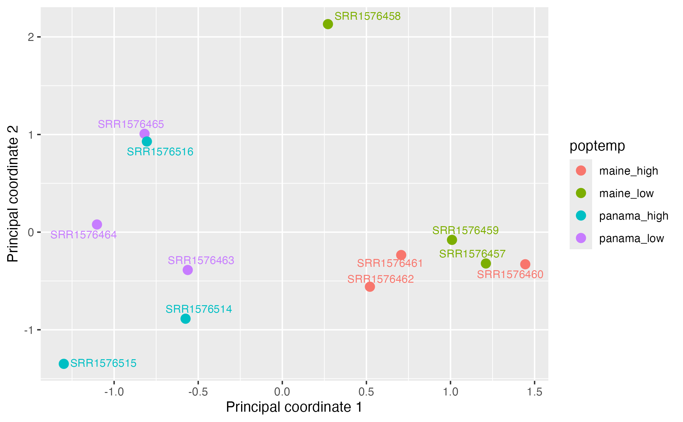
While there is clearly separation according to geographic along the first prinicipal coordinate (i.e. MDS) axis, one sample from the Maine-low temperature treatment (SRR1576458) is a bit separated from all other samples on the second axis. While it is hard to know exactly what might be the cause of this, one of the strengths of limma is that it has the option to assign "quality weights" to samples in order to down-weight samples that exhibit more outlier-like behavior. We will demonstrate this below.
8. Create design matrix
At the heart of linear modeling are design matrices that specify boolean variables for the intercept, and additional factors, and limma requires such a matrix for performing differential expression analysis. Our first analysis is going to focus on a one-factor model, in which we ignore geography and look at the effects of low and high temperature treatments. We make a design matrix for this analysis as follows:
| row number | (intercept) | templow |
|---|---|---|
| 1 | 1 | 1 |
| 2 | 1 | 1 |
| 3 | 1 | 1 |
| 4 | 1 | 0 |
| 5 | 1 | 0 |
| 6 | 1 | 0 |
| 7 | 1 | 1 |
| 8 | 1 | 1 |
| 9 | 1 | 1 |
| 10 | 1 | 0 |
| 11 | 1 | 0 |
| 12 | 1 | 0 |
The row number references the row in the sample table, and thus the associated sample id, while the boolean variable templow indicates which samples have received the low temperature treatment (i.e. those where the value in the matrix is 1).
9a. Running limma
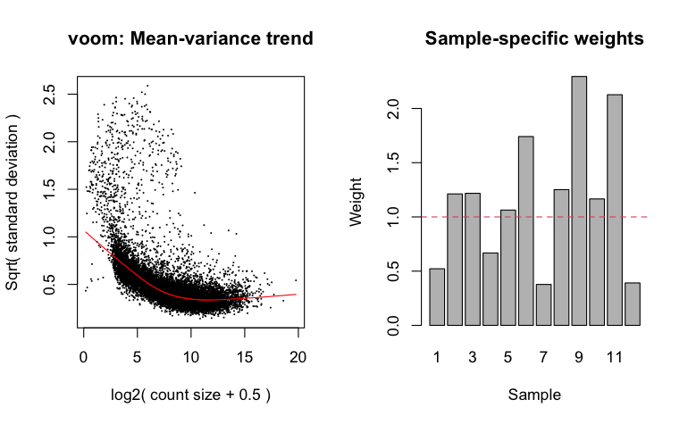
After creating the design matrix object, the standard approach is to next run limma voom on the DGE object. This step is a prelude to fitting linear models, and involves transforming count data to log-transformed counts per million (CPM), estimating the gene-wise relationship between mean and variance of expression, and calculating "observation-level precision weights", which are estimates of precision for individual genes that are then used subsequently by the lmFit function (see below) that fits linear models.
A better solution to this problem is to apply weights to samples such that outlier samples are down-weighted during differential expression calculations. Limma voom does this by calculating "empirical quality weights" for each sample. Note that we don't specify a normalization method becaues the data have already been normalized with TMM.
9b. Running limma with sample quality weights
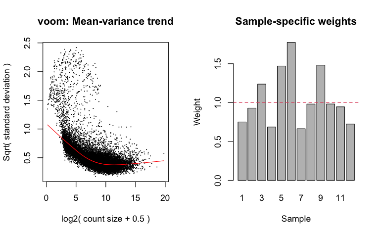
To estimate quality weights for use in downstream analysis, instead of using the standard voom function, we use voomWithQualityWeights.
Most bulk RNA-seq differential expression analysis packages need to fit a mean-variance relationship--which is used to adjust estimated variances-- and the voomWithQualityWeights command generates a plot of this relationship as well as a bar plot of the weights assigned to each sample.
NOTE: we have already applied TMM normalization, thus why normalization.method is set to "none".
10. Run the linear model fitting procedure
The next step in differential expression analysis with limma is to fit the linear model specified by the design matrix, in this case design_temp, and estimate fold changes and standard errors. The standard errors being estimated are for the coefficients of the linear model that is being fit. We do this with the lmFit function.
11. Then apply the empirical bayes procedure:
Given the typically small number of biological replicates in a bulk RNA-experiment, estimates of gene-wise dispersion (i.e. variance) of expression estimates will be noisy. Noisy, inaccurate disperion estimates will produce noisy, inaccurate estimates of linear model coefficients, leading to less robust tests for differential expression. For this reason, all bioinformatics tools for performing differential expresssion involve a step in which the standard errors estimates are adjusted. This adjustment is predicated upon the reasonable assumption that genes with similar expression levels should have similar variances. We can observe this general pattern in the mean-variance relationship that estimated (and plotted) when we run voomWithQualityWeights. This adjustment of standard errors being with "shrinkage" of gene-wise variances, a process in which those variances are "shrunk" towards the fitted curve in the mean-variance relationship--genes whose dispersion is further away from the fitted line have their variances "shrunk" more, those that are closer are "shrunk" less--and standard errors are recalcuated from these "shrunk" variances. Different tools do this is slightly different ways. In limma, this is done with the eBayes function. eBayes takes as input the fit object created with lmFit , and computes moderated t-statistics, moderated F-statistics, and log-odds of differential expression by empirical Bayes moderation (i.e. "shrinkage") of the standard errors. We use the robust=TRUE setting to leverage the quality weights such that the analysis is robust to outliers.
12. Get summary table and make volcano plot
One can then get a quick and dirty summary of how many genes are differentially expressed, setting the FDR threshold,where the "fdr" and "BH" methods are synonymous for Benjamini Hochberg adjusted p-values.
| test result | (Intercept) | templow |
|---|---|---|
| Down | 250 | 1589 |
| NotSig | 511 | 9990 |
| Up | 12546 | 1728 |
Remember, the way the design matrix has been set up means that the intercept = the mean expression for the high temperature condition, so that test results are interpreted as follows:
- Down = the low temperature condition is down-regulated relative to the high-temperature condition (i.e. LFC <0)
- Up = the low temperature condition is up-regulated relative to the high-temperature condition (i.e. LFC >0)
- NotSig = the null hypothesis that expression does not differ between the low and high temperature conditions was not rejected
In other words, logfold change is being calculated relative to the "reference" condition defined by the intercept, which is high temperature, so log-fold change calculations will have low temperature expression in the numerator and high temperature expression in the denominator. Overall, (1589+1728)/13307 or ~ 24.9% of genes are differentially expressed as a function of temperature treatment, without considering the effect of population.
Why is the intercept significant for nearly all genes? Remember, the intercept estimates the baseline expression level for the high temperature condition, such that the null hypothesis is that gene expression in the high temperature condition does not differ from zero. It is a trivial and, frankly, uninteresting hypothesis to test, such that we generally don't pay attention to results for the intercept.
We can also make a quick and dirty volcano plot, where the x-axis is log-fold change, and the y-axis is -log10(Pvalue) using limma's volcanoplot function:
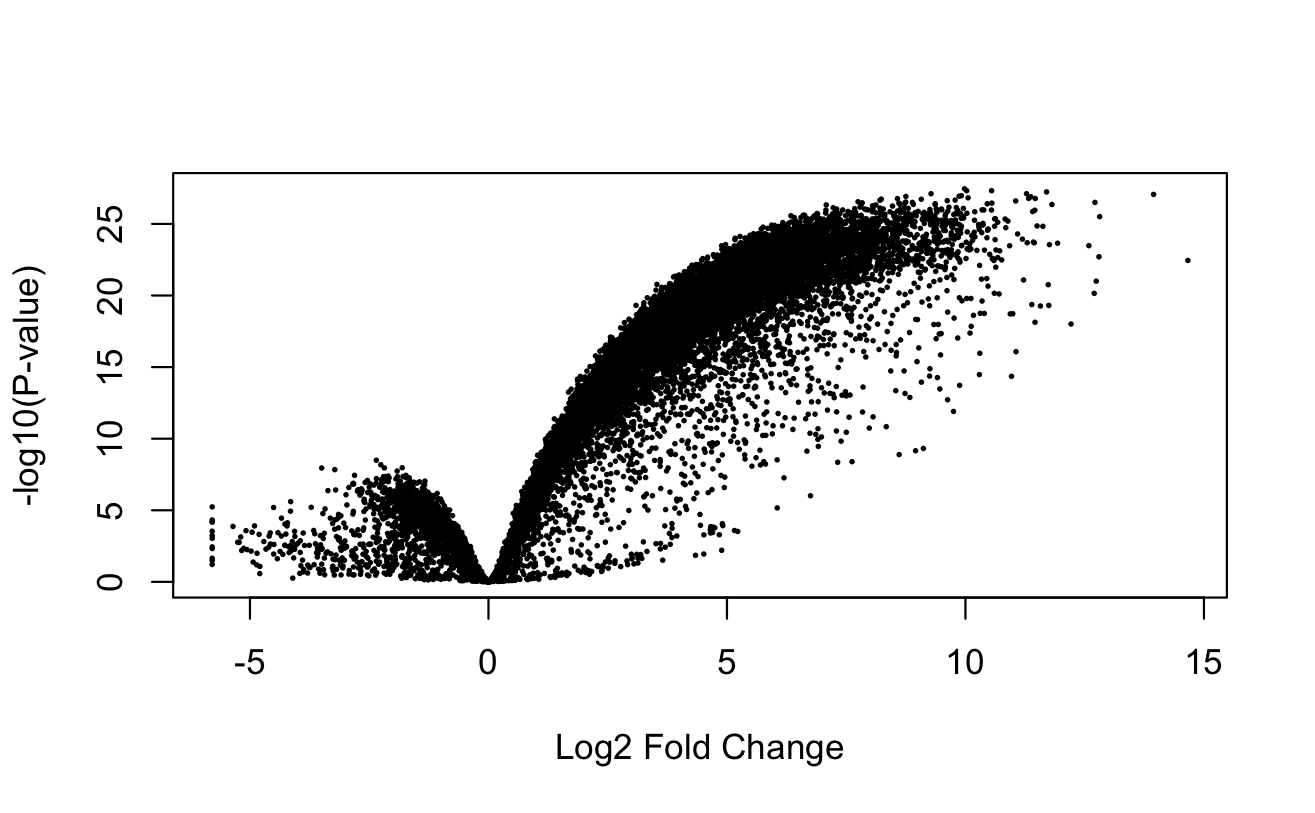
Remember, the coefficient indexed by 0 is the intercept, which we are less interested in. Thus, 1 would refer to templow. The volcano plot suggests there are far more genes that are up-regulated in the low temperature condition (i.e. with log-fold change > 0) than there are genes up-regulated in the high temperature condition.
13. Explore top 10 DE genes (ordered by p-value):
                               logFC  AveExpr         t      P.Value    adj.P.Val        B
FBgn0038819_Cpr92F          2.473527 6.201774  24.28881 1.306910e-13 1.739105e-09 21.29258
FBgn0028544_Vajk3           1.675184 4.029281  21.90298 6.069753e-13 3.524528e-09 19.66813
FBgn0267681_lncRNA:CR46017 -3.974938 1.044005 -21.50807 7.945880e-13 3.524528e-09 16.80878
FBgn0031940_CG7214          2.198970 7.945664  20.75054 1.349821e-12 4.490516e-09 19.14847
FBgn0038702_CG3739         -2.869172 6.514652 -20.49734 4.414988e-12 1.175005e-08 18.01975
FBgn0014454_Acp1            2.231834 7.638125  17.79441 2.089853e-11 3.997808e-08 16.54909
There are several columns in the output:
- the gene name (the row name)
- log-fold change
- AveExpr, the average expression across samples
- t the t-statistic for the underlying t-test
- P.value, the raw P-value
- adj.P.Val, the Benjamini-Hochberg FDR-adjusted p-value, aka a q value
- B is the B-statistic, i.e. the log-odds that the gene is differentially expressed.
14. Create results table for all genes
topTable used with default arguments reports DE results for the 10 most highly significant differentially expressed genes. However, one often needs the results for all genes, even those for which there was no significant DE. This information is useful for querying specific hypothesized candidate genes--and it may be interesting that some candidates are not differntially expressed--but is also useful for common data visualizations such as MA plots or volcano plots. To get the results for all genes you can use the topTable function but specify a p-value threshold of 1.
NOTE: one must explicitly specify the coefficient for the factor of interest. In this case, as revealed in the summary table above, it is templow.
where:
coeff = the coefficient or contrast you want to extract
number = the max number of genes to list
adjust = the P value adjustment method
resort.by determines what criteria with which to sort the table
DE analysis: a more complicated, 2-factor design
Extending limma to analyze more complex designs, such as when considering two factors, temperature and population, is relatively straightforward. A key part is to specify the design matrix properly. For the 2-factor design, one would do this as follows.
15. build design matrix for 2-factor model
population <- factor(sample_info$population,levels=c("maine","panama"))
temperature <- factor(sample_info$temp, levels=c("high","low"))
design_2factor <- model.matrix(~population+temperature)
design_2factor
| row number | (intercept) | populationpanama | temperaturelow |
|---|---|---|---|
| 1 | 1 | 0 | 1 |
| 2 | 1 | 0 | 1 |
| 3 | 1 | 0 | 1 |
| 4 | 1 | 0 | 0 |
| 5 | 1 | 0 | 0 |
| 6 | 1 | 0 | 0 |
| 7 | 1 | 1 | 1 |
| 8 | 1 | 1 | 1 |
| 9 | 1 | 1 | 1 |
| 10 | 1 | 1 | 0 |
| 11 | 1 | 1 | 0 |
| 12 | 1 | 1 | 0 |
Then, you would proceed with DE analysis in a similar fashion as with the single factor experiment described above. Notice that we have specified the levels of temperature such that low is second, which results in "templow" being the dummy variable with which to fit the coefficient for temperature.
16. Run limma with quality weights with 2-factor design matrix
vwts_2factor <- voomWithQualityWeights(DGE, design=design_2factor,normalize.method="none", plot=TRUE)
fit_2factor <- lmFit(vwts_2factor,design_2factor)
fit_2factor <- eBayes(fit_2factor,robust=TRUE)
summary(decideTests(fit_2factor,adjust.method="fdr",p.value = 0.05))
| test result | (Intercept) | populationpanama | temperaturelow |
|---|---|---|---|
| Down | 249 | 765 | 2259 |
| NotSig | 565 | 11625 | 8646 |
| Up | 12493 | 917 | 2402 |
There are now (2259+2402)/13307 or ~ 36.4% of genes are differentially expressed as a function of temperature after partitioning variation among temperature and population-level effects. In essence, accounting for population-level variation provided greater power in detecting the effects of temperature, as in the above 1-factor test, only 24.9% of genes were differentially expressed with respect to temperature.
17. Get results table for all genes
As before, we can get the entire table (including those that do not show significant DE). NOTE: when we fit models with limma with a multi-factor design there are now two possible coefficients to select. Because we are interested in the effects of temperature, we specify temperaturelow. If we wanted to look at genes with differential regulation with respect to population, we would have to specify populationpanama.
Specifying particular comparisions: data subsetting
In a simple experiment where you have two groups of samples, with each assigned to one of two different conditions, following a workflow akin to the "vanilla one factor" one described above is a perfectly reasonable. For example, if there was no second "population" factor, such as if flies had only been collected from Panama and subjected to either high or low temperature treatments. However, not all experiments are that straightforward. For example, you may one factor, and several levels for that factor, and you might only be interested in specific comparisons. Imagine a case where there are three temperature levels: low, medium and high, and you are only interested in changes relative to "low". In other words, you might only want to test for DE between a) medium and low and b) high and low. Or, in a two factor experiment such as in our example data, you might only be interested in testing for changes between high and low temperature within each population. One way to perform these tests is to:
- subset the DGE to only include samples from the conditions of interest
- create a design matrix from this subsetted data, and
- run the DE testing with limma per the "vanilla experiment
We will demonstrate how this is done for carrying out a DE test for high versus low temperature only within the Panama population
subset the data
subset the DGE
panama_samples<-sample_info$sample[sample_info$population=="panama"]
panama_DGE <- DGE[,panama_samples]
subset the sample info table
We do this by selecting rows with "panama" for the value of the population factor, and include all columns. Because limma and edgeR work with data frames and not tibbles, we use base R code for doing this.
panama_sample_info <-sample_info[sample_info$population=="panama",]
panama_sample_info$temp<-factor(panama_sample_info$temp, levels=c("high","low"))
panama_sample_info
| row number | sample | population | temp | pop_temp |
|---|---|---|---|---|
| 7 | SRR1576463 | panama | low | panama_low |
| 8 | SRR1576464 | panama | low | panama_low |
| 9 | SRR1576465 | panama | low | panama_low |
| 10 | SRR1576514 | panama | high | panama_high |
| 11 | SRR1576515 | panama | high | panama_high |
| 12 | SRR1576516 | panama | high | panama_high |
Notice that the row numbers are preserved from the original sample table, i.e. they are not re-numbered on the fly to start at 1.
create design matrix for subsetted data
do DE testing on Panama samples
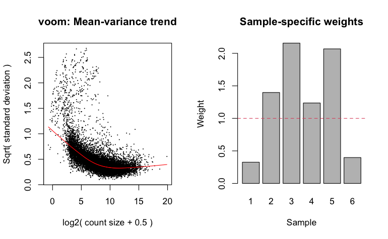
vwts_panama <- voomWithQualityWeights(panama_DGE, design=panama_design_temp,normalize.method="none", plot=TRUE)
panama_fit=lmFit(vwts_panama,panama_design_temp)
panama_fit=eBayes(panama_fit,robust=TRUE)
summary(decideTests(panama_fit,adjust.method="fdr",p.value = 0.05))
| test result | (Intercept) | templow |
|---|---|---|
| Down | 1481 | 1964 |
| NotSig | 1232 | 11013 |
| Up | 12527 | 2263 |
topTable(panama_fit, adjust="BH",resort.by="P")

          logFC  AveExpr         t      P.Value    adj.P.Val        B
Acp1     2.324353 7.742532  26.98556 1.297966e-11 1.722261e-07 17.08139
Cpr92F   2.473170 6.188566  25.67331 2.260185e-11 1.722261e-07 16.55697
tim     -1.516393 6.111509 -21.04818 2.041175e-10 7.080602e-07 14.51690
CG43732  4.143109 2.740078  20.83128 2.288273e-10 7.080602e-07 13.29214
Acyp     2.304751 3.771257  20.80282 2.323032e-10 7.080602e-07 14.16458
TM4SF    1.245547 5.012359  16.88155 2.295124e-09 5.675822e-06 12.13905
CG40472  2.431640 5.644105  20.06151 2.607005e-09 5.675822e-06 12.10037
twi     -1.779439 4.385314 -16.19768 3.599106e-09 6.268029e-06 11.68599
PPO1    -1.690476 4.421855 -16.05957 3.949836e-09 6.268029e-06 11.59834
Vajk3    1.485155 4.050126  15.95085 4.252039e-09 6.268029e-06 11.51536
all_genes <- topTable(fit_2factor, adjust="BH",coef="temperaturelow", p.value=1, number=Inf ,resort.by="P")
all_genes$geneid <- row.names(all_genes)
Specifying particular comparisions: linear contrasts
Under the hood, limma fits linear models to patterns of expression across conditions, such that, when it performs differential expression tests, it is testing the null hypothesis that the coefficient for a particular term in the linear model is equal to zero. limma leverages the design matrix to build the model from which statistical tests will be performed on the coefficients of that model. In the simple case of the dataset restricted to samples from Panama, our model is:
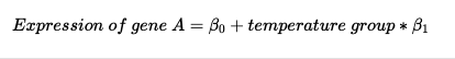
In the above formula, temperature group references the group coding for the temperature factor in the design matrix. Because "high" is the first level, it is represented in the matrix by zeroes, and "low" by ones. limma interprets this coding to assign samples to groups, and constructs a model where the first coefficient represents the mean expression of gene A, and the second coefficient represents the difference in expression between low and high temperature conditions, i.e. low-high. One of limma's big advantages is that, for complex experiments, one is able to specify arbitrary contrasts to extract and test, leveraging the full spectrum of options for linear modeling. However, doing so properly requires a thorough understanding of linear modeling. If you wish to read more about linear modeling in voom, we recommend the chapter 9 of the limma user's guide . Nevertheless, there is a straightforward syntax for specifying particular "contrasts" that reflect different biological hypotheses of interest, and without having to subset the data. We demonstrate this below.
Building a contrast design matrix
You may recall that in our original sample_info object we created a variable named pop_temp. This variable concatenation is a key part of specifying contrasts in a straightforward manner. But first, we need to assign factor levels to these combinations:
contrast_design<-model.matrix(~0+poptemp)
colnames(contrast_design) <- levels(poptemp)
contrast_design
| row number | maine_low | maine_high | panama_low | panama_high |
|---|---|---|---|---|
| 1 | 1 | 0 | 0 | 0 |
| 2 | 1 | 0 | 0 | 0 |
| 3 | 1 | 0 | 0 | 0 |
| 4 | 0 | 1 | 0 | 0 |
| 5 | 0 | 1 | 0 | 0 |
| 6 | 0 | 1 | 0 | 0 |
| 7 | 0 | 0 | 1 | 0 |
| 8 | 0 | 0 | 1 | 0 |
| 9 | 0 | 0 | 1 | 0 |
| 10 | 0 | 0 | 0 | 1 |
| 11 | 0 | 0 | 0 | 1 |
| 12 | 0 | 0 | 0 | 1 |
In this design, each value for poptemp gets a column, with ones indicating if the sample is assigned to that value. Once it has been created, we can make a contrast matrix, with named contrasts:
Mlowhispecifies a contrast (and model coefficient) for the difference in expression between low and high temperature expression in MainePlowhispecifies a contrast for the difference in expression between low and high temperature in Panama, andDiffspecifies an interaction term for evaluating whether the nature of the difference between low and high temperature depends upon geographic location, i.e. does the difference vary by geography
cont.matrix <- makeContrasts(Mlowhi=maine_low-maine_high,Plowhi=panama_low-panama_high,Diff=(maine_low-maine_high)-(panama_low-panama_high),levels=contrast_design)
cont.matrix
| Contrasts: | Mlowhi | Plowhi | Diff |
|---|---|---|---|
| Levels: | |||
| maine_low | 1 | 0 | 1 |
| maine_high | -1 | 0 | -1 |
| panama_low | 0 | 1 | -1 |
| panama_high | 0 | -1 | 1 |
Build a voom object for the contrast design
Next, we need to rebuild a voom object specifying the new design:
vwts_contrast <- voomWithQualityWeights(DGE, design=contrast_design,normalize.method="none", plot=TRUE)
do DE testing
Next we can do DE testing and extract the comparisons (i.e contrasts) of interest
run linear model fitting
fit contrasts
run empirical Bayes procedure
get summary table
We can generate a summary table as with the above examples, but also visualize overlap of significant differences between coefficients.
contrast_summary<-decideTests(fit_2factor_contrast,adjust.method="fdr",p.value = 0.05)
summary(decideTests(fit_2factor_contrast,adjust.method="fdr",p.value = 0.05))
vennDiagram(contrast_summary)
create merged results table
Because the first, second and third coefficients in the cont.matrix are for Mlowhi, Plowhi, and Diff, we can extract the results for each contrast and combine the results into a single table:
Mlowhi_results<-topTable(fit_2factor_contrast, adjust="BH",coef=1, p.value=1, number=Inf ,resort.by="P")
colnames(Mlowhi_results)<-paste("Mlowhi",colnames(Mlowhi_results),sep=".")
Mlowhi_results$geneid<-row.names(Mlowhi_results)
Plowhi_results<-topTable(fit_2factor_contrast, adjust="BH",coef=2, p.value=1, number=Inf ,resort.by="P")
colnames(Plowhi_results)<-paste("Plowhi",colnames(Plowhi_results),sep=".")
Plowhi_results$geneid<-row.names(Plowhi_results)
Diff_results<-topTable(fit_2factor_contrast, adjust="BH",coef=3, p.value=1, number=Inf ,resort.by="P")
colnames(Diff_results)<-paste("Diff",colnames(Diff_results),sep=".")
Diff_results$geneid<-row.names(Diff_results)
results_merge<-merge(Mlowhi_results,Plowhi_results,by=c("geneid"))
results_merge<-as_tibble(merge(results_merge,Diff_results,by=c("geneid")))
Once this merged table is created, one can query it using tidyverse table parsing to ask particular questions of interest. For example, which genes are up-regulated in high temperature conditions in a parallel fashion between Panama and Maine? To do this, you would want to identify genes where there is a non-significant interaction term, log-fold change is negative in both regions (remember, the contrast and factor levels mean it's low-high, so negative values mean up-regulation with high temperature), and significant for both regions, assuming an FDR level of 0.05.
parallel_high_upreg_genes <-results_merge %>% filter(Diff.adj.P.Val > 0.05) %>%
                  filter(Plowhi.adj.P.Val <=0.05) %>%
                  filter(Mlowhi.adj.P.Val <=0.05) %>%
                  filter(Plowhi.logFC < 0) %>%
                  filter(Mlowhi.logFC < 0)
Questions/Troubleshooting
1. My Nextflow run is failing while running on the Cannon cluster! What should I do?
Please check the following:
- Make sure you have Nextflow installed and loaded (if in a conda environment)
- Make sure your environment includes java, which needs to be installed in the same conda environment or, if Nextflow is in your base environment, that you load java with
module load jdk. - Check that your config file is submitting jobs to the correct partition. You may instead consider using the
-profile cannonoption, which will use the default config file for the Cannon cluster. - If you are still having issues, consider contacting us
2. What is a good sample size for differential expression analysis?
The more biological replicates per condition, the greater the statistical power to detect differential expression. At a bare minimum, for tools like limma to work properly, one needs a minimum of three biological replicates per condition, or combination of conditions, e.g. temperature x geographic region in the case of our example data.
3. How do I deal with drastically varying quality and read depth across my samples?
Samples wih low quality can typically be flagged with alignment base QC metrics, and limma voom can adjust the contribution of individual samples in inverse proportion to their "quality" as inferred by their location in reduced dimension space relative to other samples. However, if very few reads align to the transcriptome or there are other indicators of poor quality, the researcher will have to make a judgement call about excluding samples. Regarding read depth, one intrinsically expects read depth variation simply due to variation in expression across genes. That aside, a high quality sequencing library with roughly 15 million reads should produce good expression estimates, assuming the genome annotation is also reasonably accurate and complete. But, if many reads don't align, this will reduce coverage depth across the transcriptome and reduce statistical power for detecting DE. This becomes more of an issue when the low quality samples are biased towards particular conditions that are in the experiment.